Field story 01 · the Kosi flood, September 2025 · four acts
One Flood: From Raw Pixels to a Relief Plan
In late September 2025 the Kosi barrage released record water and north Bihar went under. This is that flood, worked end to end with almost nothing but NumPy and SciPy: find the water, count who is under it, see what got cut off, and decide where the relief camps go. The flood was pixels. The disaster was a graph. The response is an equation.
Where is the water? (the satellite that ignores clouds)
The problem with monsoon floods
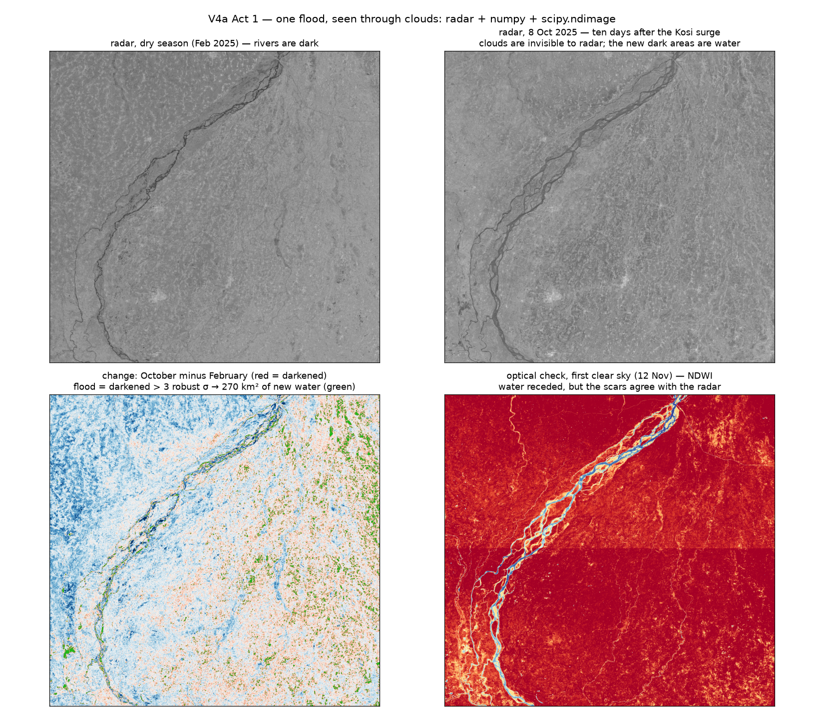
The one moment you desperately need satellite photos is exactly the moment the sky is solid cloud. Ordinary imagery is useless mid-flood. Radar is not: it shines its own signal through the clouds, and water reflects that signal away, so flooded land turns dark. We used the radar pass from October 4, ten days into the event, and a dry February pass as the "normal" reference.
The honest failure first
We tried the textbook trick, Otsu's automatic threshold, and it failed. Water was only 2% of the scene, so the "optimal" split landed inside the dry land's own shades. Keep this in the talk. The fix is to stop looking for "dark" and start looking for "newly dark": subtract February from October and flag whatever darkened more than the speckle noise can explain.
How it works
Clean both radar images with a median filter (the classic anti-speckle move). Subtract. The difference image has a natural noise level, which we measure with the median and the median absolute deviation. Anything that darkened by more than three of those robust sigmas is flood. Then the usual cleanup: morphology wipes the specks, and a size filter drops anything smaller than a hectare.
Flood = got darker than noise can explain. The threshold calibrates itself from the scene; no magic numbers travelled in.
diff = median_filter(october, 5) - median_filter(february, 5)
flood = diff < np.median(diff) - 3 * mad(diff)     # newly dark = new water
What it means
Flood mapping through clouds is not a satellite-agency monopoly. It is a subtraction, a median filter, and a threshold that explains itself — running in a container on public data, the week it matters.
Who is under it? (every rooftop asks one question)
Why this matters
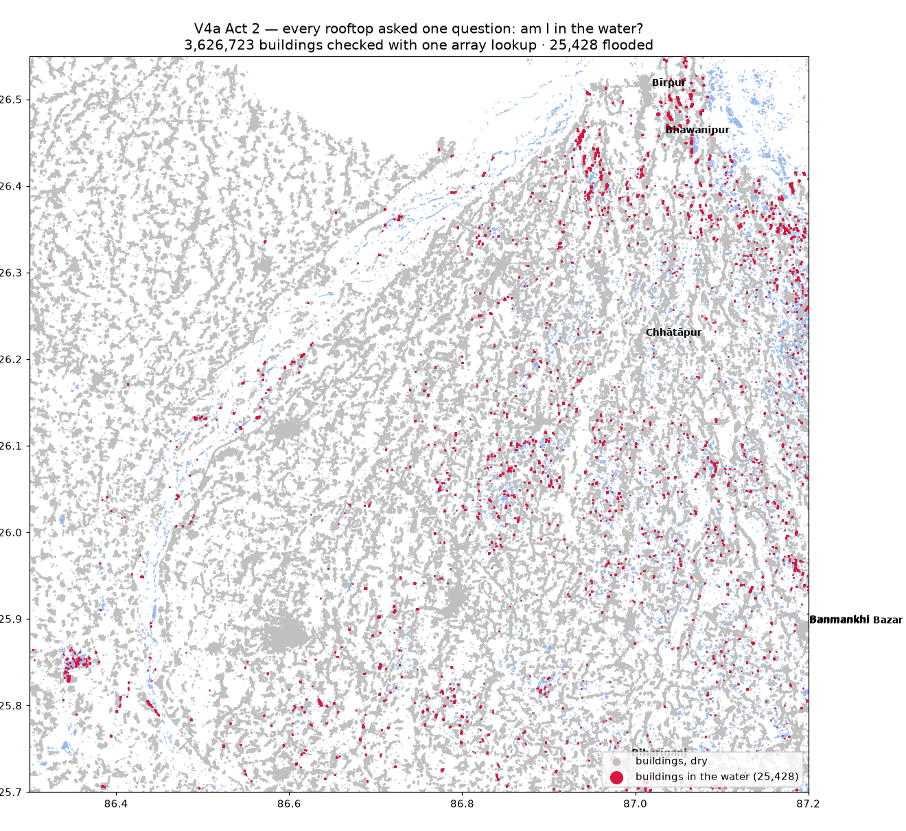
"270 km² flooded" is a headline. It is not a plan. A plan needs to know how many homes, and in whose villages. We have 3.6 million real rooftops for this belt from the scaling talk. Each one asks the flood grid a single question: am I in the water? That is one array lookup per building — all of them together take under a second.
What came back
- 25,428 buildings in the new water.
- Seven settlements with flooding within 2 km, led by Bihariganj, Banmankhi and Bhawanipur — the historical Kosi flood belt, found by arithmetic, not by memory.
- A per-village count ready for the district's situation report.
How it works
The flood mask is a grid. A building's coordinates convert to a row and column with two subtractions and two divisions. That's it. No spatial join, no database, no waiting.
When one side of a spatial question is a grid, the join is free.
row = ((north_edge - lat) / cell).astype(int)
col = ((lon - west_edge) / cell).astype(int)
underwater = flood[row, col]                  # 3.6M answers, instantly
What it means
Exposure assessment — the first report every disaster authority writes — is a grid lookup away once the water is mapped. The bottleneck was never the computation. It was knowing the computation is this small.
What got cut off? (the disaster is the disconnection)
Why this matters
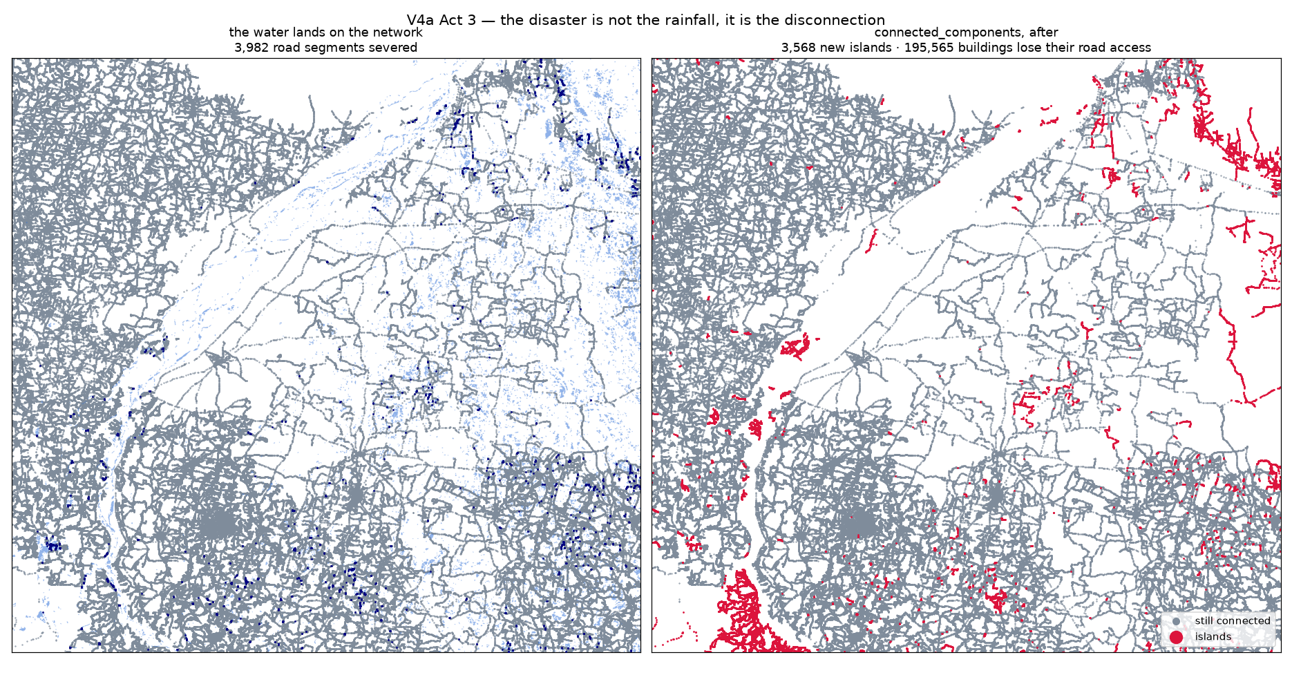
People survive standing water. What kills is the ambulance that cannot arrive and the supplies that cannot leave. So the sharpest question is not "what is wet" but "which places can no longer be reached". We took the belt's road network, deleted every segment that touches the new water, and asked the graph how many pieces it fell into.
What came back
- Before: 134 pieces. After: 3,702 — the flood carved 3,568 new islands out of the road network.
- The big towns stayed connected; they sit on highways.
- The victims are on the lanes: 195,565 buildings lost their road access, computed by giving every building the fate of its nearest road point.
How it works
Roads are a sparse matrix (the scaling talk's trick). Severing the flooded segments is one boolean mask on the edge list. Connected components then labels every island in a third of a second, before and after, and the difference is the damage report.
Rainfall is weather. Disconnection is disaster. Only the graph can tell them apart.
g_after = graph_from(edges[~edge_touches_water])
n_before, _ = connected_components(g_before)   # 134 pieces
n_after, labels = connected_components(g_after) # 3,702 pieces
What it means
Two runs of one function turn a weather map into an access map. If you only have budget for one analysis in the first hours of a flood, run this one — it tells you where the boats need to go.
Where does the relief go? (the response is an equation)
Why this matters
Relief camps get placed under pressure, by instinct, in whichever towns officials can name fastest. But "place camps so affected people travel least, on the roads that still exist" is a solvable problem — the same facility mathematics from the Map-is-a-Matrix talk, now with the surviving road network as the distance oracle.
What came back
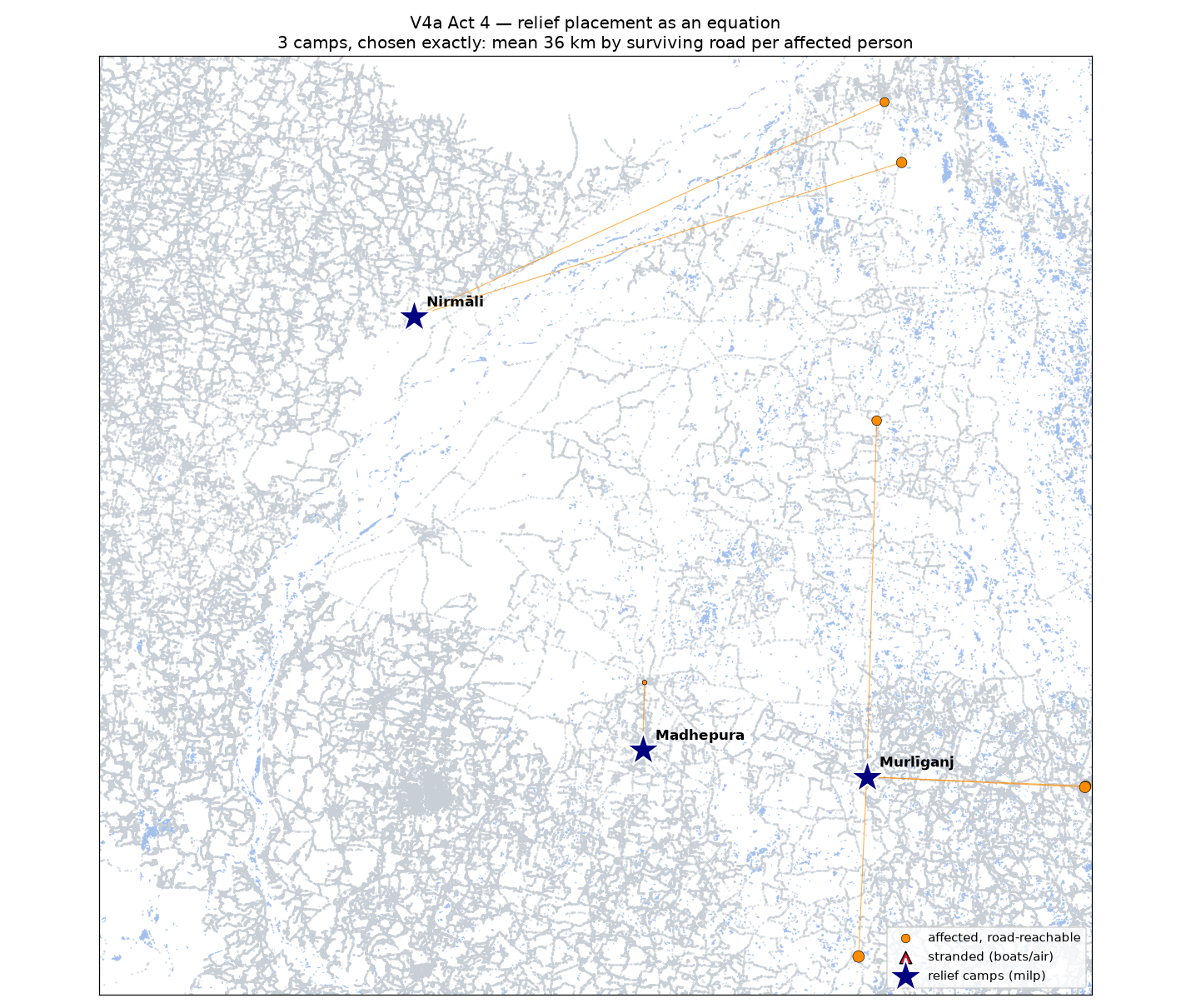
- Camps at Nirmali, Murliganj and Madhepura — the last being exactly the district HQ a collector would choose, derived instead of assumed.
- Mean road distance to relief: 36 km per affected person, provably the best three-camp answer.
- Stranded settlements flagged separately: they need boats, not camps.
How it works
Dijkstra on the surviving network gives true travel distances from every candidate town to every affected one. A small integer program then chooses the three camps that minimise population-weighted distance — solved exactly, in under a second, by the solver that ships inside SciPy.
The equation doesn't outrank local knowledge. It hands local knowledge a defensible starting point, with a number attached.
dist = dijkstra(surviving_graph, indices=candidate_towns)
res = milp(c=weighted_dist, constraints=[assign_once, open_exactly_3, linking],
           integrality=all_binary)          # exact, < 1 s
What it means
From raw radar to a camp plan: four scripts, one container, no GIS desktop, no cluster. The flood was pixels. The disaster was a graph. The response is an equation. That is the whole talk, and it ran on a real flood.
Where the story continues
The flood has a fifth question: whose land went under water — the compensation problem. That one needs the cadastral records, and they bring their own trouble. It gets its own story: Whose Land Flooded?