Talk 02 · engineering · SciPy, sparse matrices, and memory-aware Python
When GeoPandas Stops Scaling
One innocent question drives this whole talk: find the nearest road for every building in Bihar. That is 38 million buildings against 11 million road points. The obvious approach needs 69 days of computing and a table no machine on earth can hold. The right approach takes 5 seconds on one laptop. Nothing about the question changed. Only its shape did.
38 million real buildings (and the lie we caught before it shipped)
Where it comes from
The buildings are real: Google's Open Buildings dataset, traced from satellite photos. We streamed 59.6 million rooftops for the wider region straight out of compressed files, no database, no server. The roads are every OSM road in the region, cut from the full 1.7 GB India file in one pass. Total setup: about 2.5 GB of downloads, cached once.
The war story
Our first road-access map had a thick black band across the top: millions of buildings apparently 3 km from any road. The truth: the building data covers Nepal, but the India road file stops exactly at the border. Two datasets, two silent boundaries. Until you clip them to the same shape, the statistics lie with a straight face.
How the clip works at this scale
Checking 60 million points against a state boundary, point by point, would crawl. So we drew the boundary once onto a fine grid, like a stencil, and then each building just looks up which grid cell it falls in. One drawing, 60 million instant lookups.
Which is the whole talk in miniature: don't do the slow thing 60 million times. Do the slow thing once, then make the 60 million things cheap.
The obvious way is correct, fast, and hopeless
Why this matters
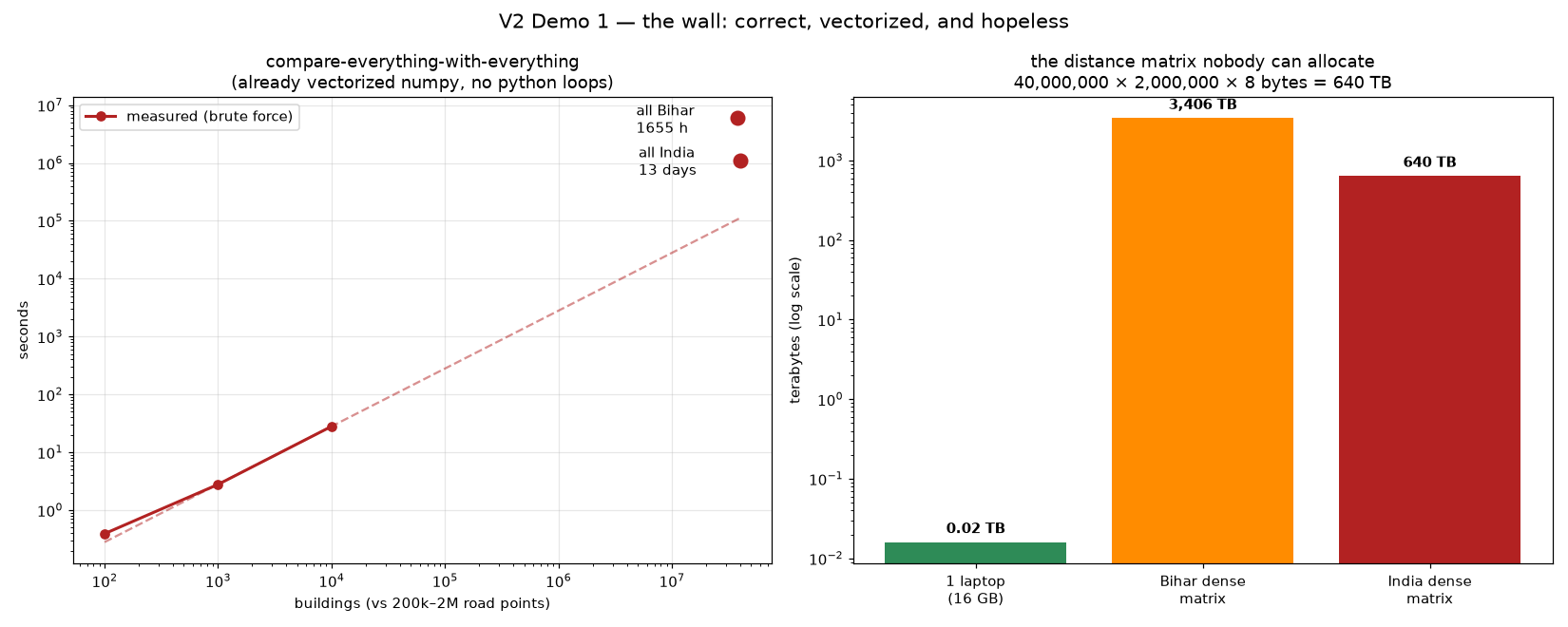
Every scaling disaster starts as working code. Compare each building with each road point, keep the closest: correct, easy to read, and it even runs fast on a test sample. The trap is that "compare everything with everything" grows as a multiplication. Double the buildings and double the roads, and the work goes up four times.
When you'll meet this wall
- The pilot worked: 10,000 rows in the demo, 40 million in production.
- A join between two big point sets: customers × stores, incidents × assets.
- Anything with a loop over one dataset inside a loop over another.
- The day someone says "just run it overnight" and overnight isn't enough.
How bad is it, measured honestly
We didn't strawman it. The comparison code is properly vectorized numpy, no Python loops, crunching 74 million pairs every second. That's genuinely quick. And at 38M × 11M pairs it still needs 1,655 hours: 69 days. Storing the distances as a table would take 3,406 terabytes. The all-India version, 40M buildings × 2M road points, is 13 days and 640 terabytes.
The recurring visual: 40,000,000 × 2,000,000 = absolutely not. No amount of "faster code" fixes a shape that multiplies.
d2 = ((buildings[:, None, :] - roads[None, :, :]) ** 2).sum(-1)
nearest = d2.argmin(1)      # correct. vectorized. 69 days.
What it means
When your spatial code is slow, the first question is not "how do I make this loop faster?" It is "what is the shape of this computation, and does it multiply?" If it multiplies, stop optimizing and change the shape.
Same question, 5 seconds (the tree that skips the work)
Why this matters
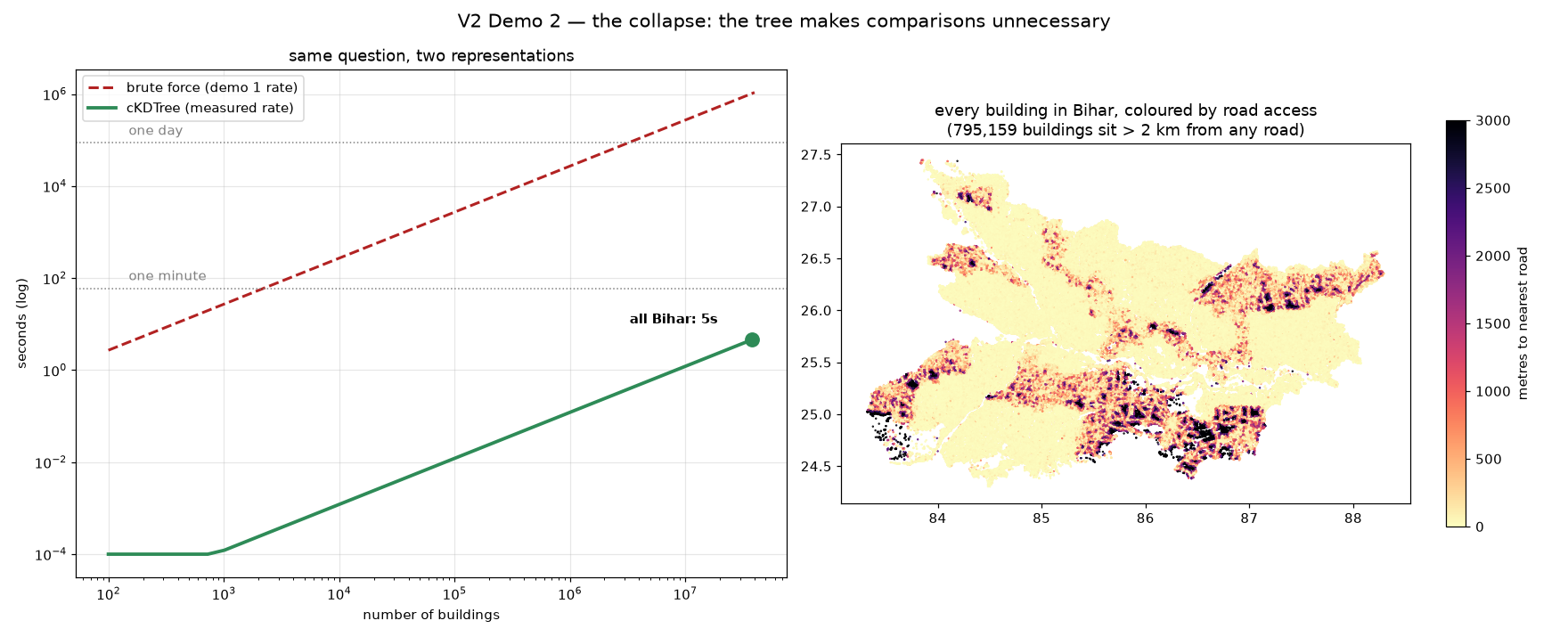
The k-d tree from talk one comes back, but at scale the point lands differently. The tree doesn't compare faster. It refuses to make almost every comparison, because sorting space in advance tells it which comparisons could never win. The 69-day job collapses to seconds, on the same machine, with the same data.
The supporting cast
- Chunking: query 2 million buildings at a time, so memory stays flat instead of ballooning.
- All 16 cores: one argument (
workers=-1) turned a 2.2 s query into 0.2 s. - float32: half the bytes per coordinate. At 38M points, "half" is real money.
- Measure memory: the whole run fits in 2.6 GB. A phone could nearly do this.
What actually happened
Build the tree on 11.2 million road points: 2 seconds. Ask it the nearest road for all 38.2 million buildings, in chunks, on all cores: 5 seconds. That is roughly 1.25 million times faster than the wall in demo 1, and the "impossible" all-India job becomes about six seconds of compute. As a bonus, the answers are a planning map: half of Bihar's buildings are within 30 metres of a road, and 795,159 of them sit more than 2 km from one.
Nothing got faster. Almost everything became unnecessary. That is what a good representation does.
tree = cKDTree(road_points)                 # sort space once: 2 s
dist, idx = tree.query(chunk, workers=-1)   # all of Bihar: 5 s total
What it means
Before reaching for a bigger machine, a cluster, or "we need Spark", ask whether a smarter arrangement of the data makes the work disappear. A data structure is cheaper than a data centre.
A 15-terabyte table that fits in 226 megabytes
Why this matters
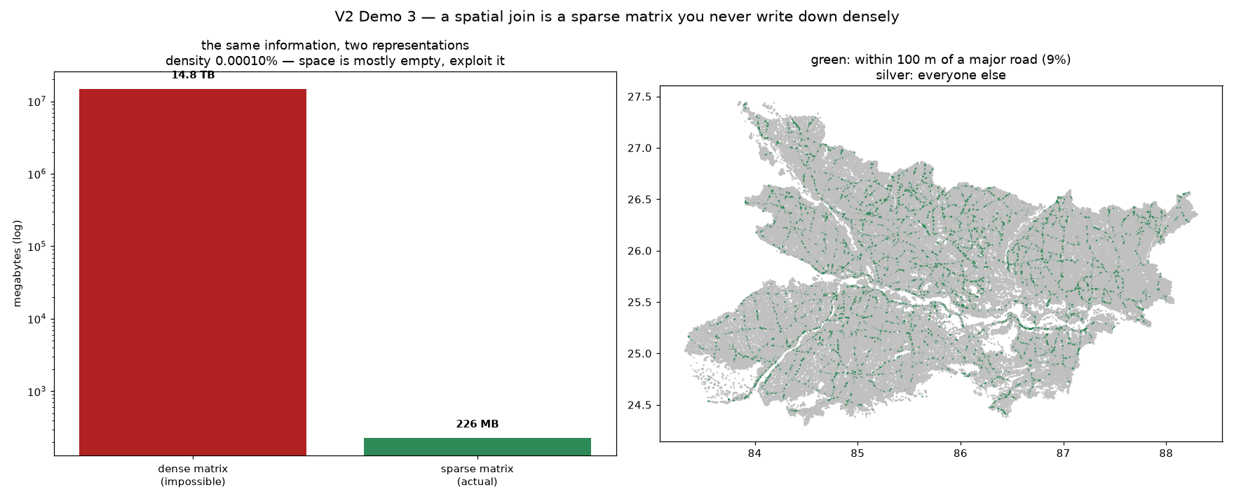
Lots of spatial questions are really relationships: which buildings sit near which roads, which sensors cover which villages, who is inside whose service area. Written as a table of buildings × roads, ours would have 23 trillion cells: 14.8 terabytes. But nearly every cell says "not close". Space is mostly empty, and that emptiness is the resource.
When you'd use this
- Coverage questions: which customers can each warehouse reach?
- Exposure questions: which homes are near which flood channels?
- Any many-to-many "near" relationship you're tempted to put in a giant cross-join.
- Feeding graphs: this matrix is one step from "walk from buildings onto the road network".
How it works
Store only the pairs that are actually close. The tree hands us, for each building, its road points within 100 metres; those pairs go into a sparse matrix that remembers position and skips the emptiness. Ours holds 14.7 million "is near" facts about a 38M × 387k relationship in 226 megabytes: the full table, minus the silence.
Only one cell in a million says anything. Store the million-to-one silence as silence.
pairs = tree.query_ball_point(buildings, r=100, workers=-1)
rel = sparse.coo_matrix((ones, (b_idx, r_idx)))   # 14.8 TB -> 226 MB
What it means
When a relationship table explodes, don't shrink your question. Notice that the table is almost entirely empty and store only what is true. Sparse matrices are how "impossible" joins become one more medium-sized file.
Every road in Bihar is one matrix (and it has 1,381 islands)
Why this matters
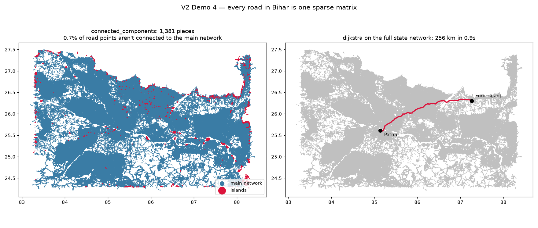
Routing engines feel like infrastructure: servers, imports, weeks of setup. But a road network is just points and connections with lengths, which is to say, a sparse matrix. The entire state's network, 11.2 million points, fits in 183 megabytes and answers questions in under a second.
When you'd use this
- Distance along roads, not as the crow flies, for every point at once.
- Data quality checks: is this "network" actually connected?
- Reachability: what can and cannot be reached from a depot, a hospital, a flood shelter.
- When OSRM is overkill and you just need answers inside a Python job.
What the matrix confessed
First question: is the road network one piece? Answer, in 0.3 seconds: no, it is 1,381 pieces. The main network holds 99.3% of the points; the rest is disconnected islands, mostly mapping gaps where someone traced a village's lanes but never joined them to the highway. Then the real test: shortest road route from Patna to Forbesganj near the Nepal border, across the whole 11-million-point graph, in 0.9 seconds: 256 km.
Connected components isn't just an algorithm. It's an X-ray for your data. Run it before you trust any network.
g = sparse.csr_matrix((lengths, (a, b)))          # the whole state: 183 MB
n, labels = connected_components(g)                # 1,381 pieces, 0.3 s
cost, pred = dijkstra(g, indices=patna, return_predecessors=True)
What it means
State-scale network analysis doesn't need a routing server. It needs a sparse matrix and two function calls. And the first thing it will tell you is the truth about your data, which is worth more than the route.
The closing slide
Every demo asked the same innocent question at a scale where the obvious answer dies. What saved it each time was never a bigger machine. It was a better shape: a tree instead of a table, silence stored as silence, a state of roads folded into one matrix.
Scaling GIS is not a hardware problem. It is a representation problem. Choose the shape that makes most of the work unnecessary, and yesterday's cluster job fits in your laptop's spare memory.